Multiple Correspondence Analysis
As an example, we are going to use here a data set which comes from a questionnaire about tea consumption.
To load the data set, click here
Presentation of the data
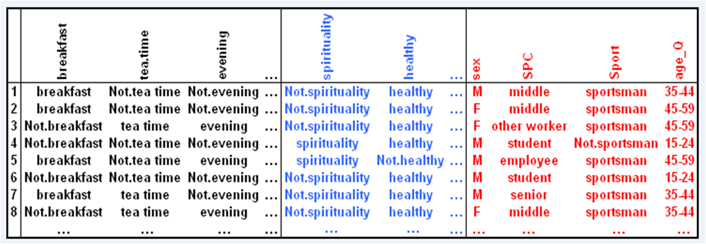
300 tea consumers have answered a survey about their consumption of tea.
The questions were about how they consume tea, how they think of tea and descriptive questions (sex, age, socio-professional category and sport practise).
Except for the age, all the variables are categorical. For the age, the data set has two different variables: a continuous and a categorical one.
To load the package and the data set, type:
library(FactoMineR)

				data(tea)
Objectives
We study individuals, variables and categories.
- Individuals'study: two individuals are close to each other if they answered the questions the same way. We will not be so interested in single individuals but rather in populations: are there groups of individuals?
- Variables and categories'study: the questions are the same as for a PCA. First, we want to see the relationship between variables and the associations between categories. Two categories are close to each other if they are often taken together. Second, we are also interested in looking for one or several continuous synthetical variables to summarize categorical ones. Third, we want to characterize groups of individuals by categories.
MCA
In this study, we will use as active variables the ones about consumption behaviour and the other variables will be added as supplementary information.
Type:
res.mca = MCA(tea, quanti.sup=19, quali.sup=c(20:36))

				plot.MCA(res.mca, invisible=c("var","quali.sup"), cex=0.7)

				plot.MCA(res.mca, invisible=c("ind","quali.sup"), cex=0.7)

				plot.MCA(res.mca, invisible=c("ind"))

				plot.MCA(res.mca, invisible=c("ind", "var"))
#tea: the data set used
#quanti.sup: vector of indexes of continuous supplementary variables
#quali.sup: vector of indexes of categorical supplementary variables
#invisible: the elements not to be plotted
#cex: character size
We can see on the individuals' scatterplot that there is no particular group of individuals. The scatterplot is quite homogeneous.
To interpret the principal components of the MCA, we are going to use extreme individuals (it is easier than using directly groups of individuals). Individuals 265 and 273 like and often drink tea in any occasion. Individuals 200 and 262 only drink tea at home, at breakfast or in the evening.
There are too many individuals to look at each one by one. That is why we need a representation of the categories.
Variables "price", "where" and "how" are much linked to both first and second dimensions. We cannot say much more and need a representation of categories to interpret these relationships better.
The first dimension opposes "tea room", "chain store+tea shop", "tea bag+unpackaged", "pub", "resto", "work" between "not friends", "not resto", "not work", "not home". It opposes regular tea drinkers to occasional ones.
The second dimension opposes "specialized shop", "unpackaged" and "upscale price" to other categories.
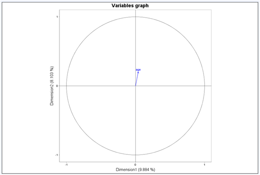
The variable "age" is not well represented. However, its correlation with the second dimension is significant (0.204) since we have a lot of individuals. Young people tend to buy tea in other places than specialized shops when old people tend to buy expensive unpackaged tea in specialized shops.
It is quite difficult to say anything about categorical supplementary variables since their categories are located at the center of the graph. However, it is possible to hide active categories and look at supplementary ones only. We then see that the categories of the variable "age_Q" are ordered from "15-24" to "+60" along the second dimension. This is in relation with the positive coordinate of the variable "age" on the second dimension.
To run a description on the dimension of the MCA, type: dimdesc(res.mca)
#res.mca: the result of an MCA
The first principal component is characterized by the variables "where", "tea room", etc. Some supplementary categorical variables are also correlated to it as "sex" and "conviviality".
Characterization by categories is similar to characterization by variables but allows more precision. For example, the coordinate of the category "tea room" is positive whereas "not tea room"'s is negative. This means that individuals whose coordinate is positive tend to go to tea rooms.
To go further
To ventilate your data, use the following option:
level.ventil
This options allows to choose the level under which the category is ventilated. The default value is 0 for no ventilation.
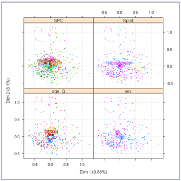
It is possible to draw confidence ellipses with the plotellipses() function:
plotellipses(res.mca,keepvar=c(20:23))
#res.mca: the result of an MCA

		#keepvar: a vector of indexes (or names) of the variables to plot


