Hierarchical Clustering on Principal Components
The following article describe in details why it is interesting to perform a hierachical clustering with principal component methods. It also gives some examples.
Husson, F., Josse, J. & Pagès J. (2010). Principal component methods - hierarchical
clustering - partitional clustering: why would we need to choose for visualizing data?. Technical report.
We are going to perform a hierarchical classification on the principal components of a factorial analysis. The dataset used is the dataset "tea" already taken to illustrate the Multiple Correspondence Analysis.
Objectives
We want to gather the 300 individuals of the dataset into a couple of clusters which would correspond to different consumption profiles.
As the variables are categorical, we will first perform an MCA then use the coordinates of the individuals on the principal components for the hierarchical classification. MCA is used as a preprocessing to transform categorical variables into continuous ones.
HCPC
The first step is to perform an MCA on the individuals.
As well as previously (see MCA page), we perform the MCA using the variables about consumption behavior as active ones.
We do not use the last axes of the MCA because they are considered as noise and would make the clustering less stable. We thus keep only the 20 first axis of the MCA which resume 87% of the information.
Type:
library(FactoMineR)

		  data(tea)
res.mca = MCA(tea, ncp=20, quanti.sup=19, quali.sup=c(20:36), graph=FALSE)
#tea: the data set used

		  #ncp: number of dimensions which are kept for the analysis

		  #quanti.sup: vector of indexes of continuous supplementary variables

		  #quali.sup: vector of indexes of categorical supplementary variables

		  #graph: logical. If FALSE, no graph is plotted
We then perform the hierarchical classification:
res.hcpc = HCPC(res.mca)
#res.mca: the result of an MCA
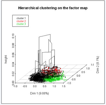
The hierarchical tree suggests a clustering into three clusters:
We get a three dimensional tree and a factorial map where individuals are coloured depending on the cluster they belong to.
Description of the clusters
Clusters can be described by:
- Variables and/or categories
- Factorial axes
- Individuals
Description by Variables and/or categories
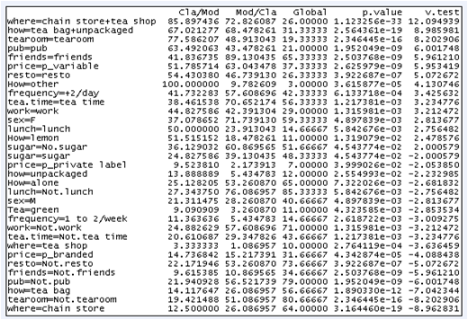
res.hcpc$desc.var$test.chi2

		res.hcpc$desc.var$category
Variables "where" and "how" are those which characterize the most the partition in three clusters.
Each cluster is characterized by a category of the variables "where" and "how". Only the categories whose p-value is less than 0.02 are used. For example, individuals who belong to the third cluster buy tea as tea bag and unpackaged tea both in chain stores and tea shops.
description by principal components
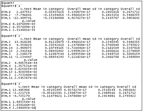
res.hcpc$desc.axes
Individuals in cluster 1 have low coordinates on axes 1 and 2. Individuals in cluster 2 have high coordinates on the second axis and individuals who belong to the third cluster have high coordinates on the first axis. Here, a dimension is kept only when the v-test is higher than 3.
description by Individuals
Two kinds of specific individuals exist to describe the clusters:
- Individuals closest to their cluster's center
- Individuals the farest from other clusters' center
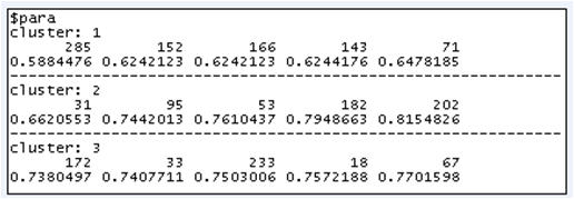
res.hcpc$desc.ind
Individual 285 belongs to cluster 1 and is the closest to cluster 1's center.
Individual 82 belongs to cluster 1 and is the farest from clusters 2 and 3's centers.
To go further
Transformation of continuous variables into categorical ones
To cut a single continuous variable into clusters:
vari = tea[,19]

		res.hcpc = HCPC(vari, iter.max=10)
		max.cla=unlist(by(res.hcpc$data.clust[,1], res.hcpc$data.clust[,2], max))

		breaks = c(min(vari), max.cla)

		aaQuali = cut(vari, breaks, include.lowest=TRUE)

		summary(aaQuali)
#iter.max: The maximum number of iterations for the consolidation
To cut several continuous variables into clusters:
data.cat = data

		for (i in 1:ncol(data.cat)){

			vari = data.cat[,i]

			res.hcpc = HCPC(vari, nb.clust=-1, graph=FALSE)

			maxi = unlist(by(res.hcpc$data.clust[,1], res.hcpc$data.clust[,2], max))

			breaks = c(min(vari), maxi)

			aaQuali = cut(vari, breaks, include.lowest=TRUE)

			data.cat[,i] = aaQuali

		}
#data: dataset with the continuous variables to be cut into clusters


